Notes on the use of data transformations. Osborne, Jason

Data transformations are commonly used tools that can serve many functions in quantitative analysis of data. The goal of this paper is to focus on the use of three data transformations most commonly discussed in statistics texts (square root, log, and inverse) for improving the normality of variables. While these are important options for analysts, they do fundamentally transform the nature of the variable, making the interpretation of the results somewhat more complex. Further, few (if any) statistical texts discuss the tremendous influence a distribution's minimum value has on the efficacy of a transformation. The goal of this paper is to promote thoughtful and informed use of data transformations.

Data transformations are the application of a mathematical modification to the values of a variable. There are a great variety of possible data transformations, from adding constants to multiplying, squaring or raising to a power, converting to logarithmic scales, inverting and reflecting, taking the square root of the values, and even applying trigonometric transformations such as sine wave transformations. The goal of this paper is to begin a discussion of some of the issues involved in data transformation as an aid to researchers who do not have extensive mathematical backgrounds, or who have not had extensive exposure to this issue before, particularly focusing on the use of data transformation for normalization of variables.

Many statistical procedures assume that the variables are normally distributed. A significant violation of the assumption of normality can seriously increase the chances of the researcher committing either a Type I or II error (depending on the nature of the analysis and the non-normality). However, Micceri (1989) points out that true normality is exceedingly rare in education and psychology. Thus, one reason (although not the only reason) researchers utilize data transformations is improving the normality of variables. Additionally, authors such as Zimmerman (e.g., 1995, 1998) have pointed out that non-parametric tests (where no explicit assumption of normality is made) can suffer as much, or more, than parametric tests when normality assumptions are violated, confirming the importance of normality in all statistical analyses, not just parametric analyses.

There are multiple options for dealing with non-normal data. First, the researcher must make certain that the non-normality is due to a valid reason (real observed data points). Invalid reasons for non-normality include things such as mistakes in data entry, and missing data values not declared missing. Researchers using NCES databases such as the National Education Longitudinal Survey of 1988 will often find extreme values that are intended to be missing. 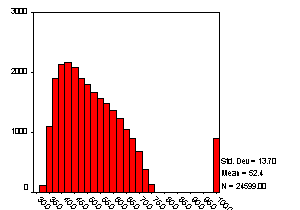In Figure 1 we see that the Composite Achievement Test scores variable (BY2XCOMP) ranges from about 30 to about 75, but also has a group of missing values assigned a value of 99. If the researcher fails to remove these the skew for this variable is 1.46, but with the missing values appropriately removed, skew drops to 0.35, and thus no further action is needed. These are simple to remedy through correction of the value or declaration of missing values.

However, not all non-normality is due to data entry error or non-declared missing values. Two other reasons for non-normality are the presence of outliers (scores that are extreme relative to the rest of the sample) and the nature of the variable itself. There is great debate in the literature about whether outliers should be removed or not. I am sympathetic to Judd and McClelland's (1989) argument that outlier removal is desirable, honest, and important. However, not all researchers feel that way (c.f. Orr, Sackett, and DuBois, 1991). Should a researcher remove outliers and find substantial non-normality, or choose not to remove outliers, data transformation is a viable option for improving normality of a variable. It is beyond the scope of this paper to fully discuss all options for data transformation. This paper will focus on three of the most common data transformations utilized for improving normality discussed in texts and the literature: square root, logarithmic, and inverse transformations. Readers looking for more information on data transformations might refer to Hartwig and Dearing (1979) or Micceri (1989).

There are several ways to tell whether a variable is substantially non-normal. While researchers tend to report favoring "eyeballing the data," or visual inspection (Orr, Sackett, and DuBois, 1991), researchers and reviewers often are more comfortable with a more objective assessment of normality, which can range from simple examination of skew and kurtosis to examination of P-P plots (available through most statistical software packages) and inferential tests of normality, such as the Kolmorogov-Smirnov test (and adaptations of this test—researchers wanting more information on the K-S test and other similar tests should consult the manual for their software as well as Goodman (1954), Lilliefors (1967), Rosenthal (1968), and Wilcox (1997), probably in that order). These can be useful to a researcher needing to know whether a variable’s distribution is significantly different from a normal (or other) distribution.

While many researchers in the social sciences are well-trained in statistical methods, not many of us have had significant mathematical training, or if we have, it has often been long forgotten. This section is intended to give a brief refresher on what really happens when one applies a data transformation.

Square root transformation. Most readers will be familiar with this procedure-- when one applies a square root transformation, the square root of every value is taken. However, as one cannot take the square root of a negative number, if there are negative values for a variable a constant must be added to move the minimum value of the distribution above 0, preferably to 1.00 (the rationale for this assertion is explained below). Another important point is that numbers of 1.00 and above behave differently than numbers between 0.00 and 0.99. The square root of numbers above 1.00 always become smaller, 1.00 and 0.00 remain constant, and numbers between 0.00 and 1.00 become larger (the square root of 4 is 2, but the square root of 0.40 is 0.63). Thus, if you apply a square root to a continuous variable that contains values between 0 and 1 as well as above 1, you are treating some numbers differently than others, which is probably not desirable in most cases.

Log transformation(s). Logarithmic transformations are actually a class of transformations, rather than a single transformation. In brief, a logarithm is the power (exponent) a base number must be raised to in order to get the original number. Any given number can be expressed as y to the x power in an infinite number of ways. For example, if we were talking about base 10, 1 is 10⁰, 100 is 10², 16 is 10^1.2, and so on. Thus, log₁₀(100)=2 and log₁₀(16)=1.2. However, base 10 is not the only option for log transformations. Another common option is the Natural Logarithm, where the constant e (2.7182818) is the base. In this case the natural log 100 is 4.605. As the logarithm of any negative number or number less than 1 is undefined, if a variable contains values less than 1.0 a constant must be added to move the minimum value of the distribution, preferably to 1.00.

There are good reasons to consider a range of bases (Cleveland (1984) argues that base 10, 2, and e should always be considered at a minimum). 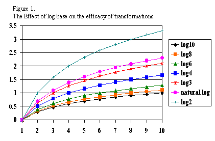For example, in cases where there are extremes of range base 10 is desirable, but when there are ranges that are less extreme, using base 10 will result in a loss of resolution, and using a lower base (e or 2) will serve (higher bases tend to pull extreme values in more drastically than lower bases). Figure 1 graphically presents the different effects of using different log bases. Readers are encouraged to consult Cleveland (1984).

Inverse transformation. To take the inverse of a number (x) is to compute 1/x. What this does is essentially make very small numbers very large, and very large numbers very small. This transformation has the effect of reversing the order of your scores. Thus, one must be careful to reflect, or reverse the distribution prior to applying an inverse transformation. To reflect, one multiplies a variable by -1, and then adds a constant to the distribution to bring the minimum value back above 1.0. Then, once the inverse transformation is complete, the ordering of the values will be identical to the original data.

In general, these three transformations have been presented in the relative order of power (from weakest to most powerful). However, it is my preference to use the minimum amount of transformation necessary to improve normality.

Positive vs. Negative Skew. There are, of course, two types of skew: positive and negative. All of the above-mentioned transformations work by compressing the right side of the distribution more than the left side. Thus, they are effective on positively skewed distributions. Should a researcher have a negatively skewed distribution, the researcher must reflect the distribution, add a constant to bring it to 1.0, apply the transformation, and then reflect again to restore the original order of the variable.

Data transformations are valuable tools, with many benefits. However, they should be used appropriately, in an informed manner. Too many statistical texts gloss over this issue, leaving researchers ill-prepared to utilize these tools appropriately. All of the transformations examined here reduce non-normality by reducing the relative spacing of scores on the right side of the distribution more than the scores on the left side.

However, the very act of altering the relative distances between data points, which is how these transformations improve normality, raises issues in the interpretation of the data. If done correctly, all data points remain in the same relative order as prior to transformation. This allows researchers to continue to interpret results in terms of increasing scores. However, this might be undesirable if the original variables were meant to be substantively interpretable (e.g., annual income, years of age, grade, GPA), as the variables become more complex to interpret due to the curvilinear nature of the transformations. 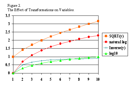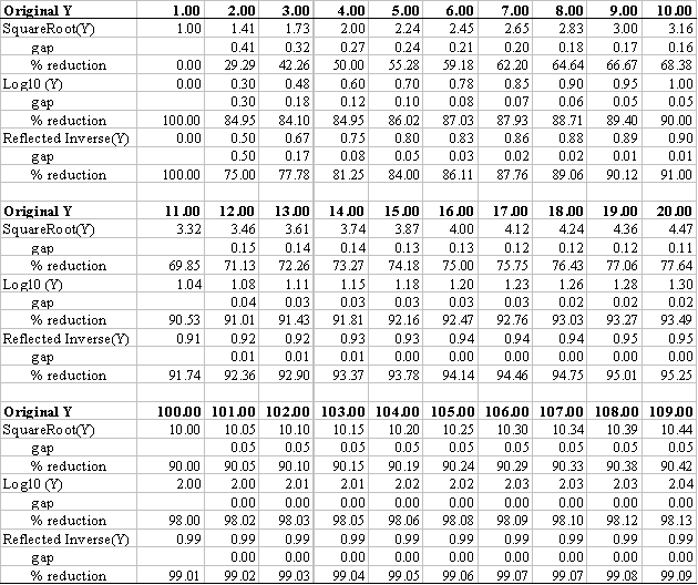Researchers must therefore be careful when interpreting results based on transformed data. This issue is illustrated in Figure 2 and Table 1.

While the original variable has equal spacing between values in Figure 2 (the X axis represents the original values), the other three lines depict the curvilinear nature of the transformations. The quality of the transformed variable is different from the original variable. If a variable with those qualities were subjected to a square root transformation, where the variable's old values were {0, 1, 2, 3, 4} the new values are now {0, 1, 1.41, 1.73, 2}—the intervals are no longer equal between successive values. The examples presented in Table 1 elaborate on this point. It quickly becomes evident that these transformations change the relative distance between adjacent values that were previously equidistant (assuming interval or ratio measurement). In the non-transformed variable, the distance between values would be an equal 1.0 distance between each increment (1, 2, 3, etc.). However, the action of the transformations dramatically alters this equal spacing. For example, where the original distance between 1 and 2 had been 1.0, now it is 0.41, 0.30, or 0.50, depending on the transformation. Further, while the original distance between 19 and 20 had been 1.0 in the original data, it is now 0.11, 0.02, or 0.00, depending on the transformation. Thus, while the order of the variable has been retained, order is all that has been maintained. The equal spacing of the original variable has been eliminated. If a variable had been measured on interval or ratio scales, it has now been reduced to ordinal (rank) data. While this might not be an issue in some cases, there are some statistical procedures that assume interval or ratio measurement scales.

Does the minimum value of a distribution influence the efficacy of a transformation?

For researchers with a strong mathematical or statistical background, the points made in this section are self-evident. However, over the years many of my students and colleagues have helped me to realize that to many researchers this point is not self-evident; further, it is not explicitly discussed in many statistical texts.

First, note that adding a constant to a variable changes only the mean, not the standard deviation or variance, skew, or kurtosis. However, the size of the constant and the place on the number line that the constant moves the distribution to can influence the effect of any subsequent data transformations. As alluded to above, it is my opinion that researchers seeking to utilize any of the above-mentioned data transformations should first move the distribution so its leftmost point (minimum value) is anchored at 1.0.

This is due to the differential effects of the transformations across the number line. All three transformations will have the greatest effect if the distribution is anchored at 1.0, and as the minimum value of the distribution moves away from 1.0 the effectiveness of the transformation diminishes dramatically.

Recalling that these transformations improve normality by compressing one part of a distribution more than another, the data presented in Table 1 illustrates this point. For all three transformations, the gap between 1 and 2 is much larger than between 9 and 10 (0.41, 0.30, and 0.50 vs. 0.16, 0.05, 0.01). Across this range, the transformations are having an effect by compressing the higher numbers much more than the lower numbers. This does not hold once one moves off of 1.0, however. If one had a distribution achored at 10 and ranging to 20, the gap between 10 and 11 (0.15, 0.04, 0.01) is not that much different than the gaps between 19 and 20 (0.11, 0.02, 0.00). In a more extreme example, the difference between 100 and 101 is almost the same as between 108 and 109.

In order to demonstrate the effects of minimum values on the efficacy of transformations, data were drawn from the National Education Longitudinal Survey of 1988. The variable used represented the number of undesirable things (offered drugs, had something stolen, threatened with violence, etc.) that had happened to a student, which was created by the author for another project. This variable ranged from 0 to 6, and was highly skewed, with 40.4% reporting none of the events occurring, 34.9% reporting only one event, and less than 10% reporting more than two of the events occurring. The initial skew was 1.58, a substantial deviation from normality, making this variable a good candidate for transformation. The relative effects of transformations on the skew of this variable are presented in Table 2.

Table 2: Variable skew as a function of the minimum score of a distribution
	Original Variable	Min = 1	Min = 2	Min = 3	Min = 5	Min = 10	Min = 100

Square Root	1.58	0.93	1.11	1.21	1.31	1.42	1.56
Log(10)	1.58	0.44	0.72	0.88	1.07	1.27	1.54
Inverse	1.58	0.12	0.18	0.39	0.67	1.00	1.50

As the results indicate, all three types of transformations worked very well on the original distribution, anchored at a minimum of 1. However, the efficacy of the transformation quickly diminished as constants were added to the distribution. Even a move to a minimum of 2 dramatically diminished the effectiveness of the transformation. Once the minimum reached 10, the skew was over 1.0 for all three transformations, and at a minimum of 100 the skewness was approaching the original, non-transformed skew in all three cases. These results highlight the importance of the minimum value of a distribution should a researcher intend to employ data transformations on that variable.

These results should also be considered when a variable has a range of, say 200-800, as with SAT or GRE scores where non-normality might be an issue. In cases where variables do not naturally have 0 as their minimum, it might be useful to subtract a constant to move the distribution to a 0 or 1 minimum.

Unfortunately, many statistical texts provide minimal instruction on the utilization of simple data transformations for the purpose of improving the normality of variables, and coverage of the use of other transformations or for uses other than improving normality is almost non-existent. While seasoned statisticians or mathematicians might intuitively understand what is discussed in this paper, many social scientists might not be aware of some of these issues.

The first recommendation from this paper is that researchers always examine and understand their data prior to performing those long-awaited analyses. To do less is to slight your data, and potentially draw incorrect conclusions.

The second recommendation is to know the requirements of the data analysis technique to be used. As Zimmerman (e.g., 1995, 1998) and others have pointed out, even non-parametric analyses, which are generally thought to be “assumption-free” can benefit from examination of the data.

The third recommendation is to utilize data transformations with care—and never unless there is a clear reason. Data transformations can alter the fundamental nature of the data, such as changing the measurement scale from interval or ratio to ordinal, and creating curvilinear relationships, complicating interpretation. As discussed above, there are many valid reasons for utilizing data transformations, including improvement of normality, variance stabilization, conversion of scales to interval measurement (for more on this, see the introductory chapters of Bond and Fox (2001), particularly pages 17-19).

The fourth recommendation is that, if transformations are to be utilized, researchers should ensure that they anchor the variable at a place where the transformation will have the optimal effect (in the case of these three, I argue that anchor point should be 1.0).

Beyond that, there are many other issues that researchers need to familiarize themselves with. In particular, there are several peculiar types of variables that benefit from attention. For example, proportion and percentage variables (e.g., percent of students in a school passing end-of-grade tests) and count variables of the type I presented above (number of events happening) tend to violate several assumptions of analyses and produce highly-skewed distributions. While beyond the scope of this paper, these types of variables are becoming increasingly common in education and the social sciences, and need to be dealt with appropriately. The reader interested in these issues should refer to sources such as Bartlett (1947) or Zubin (1935), or other, more modern sources that deal with these issues, such as Hopkins (2002, available at http://www.sportsci.org/resource/stats/index.html). In brief, when using count variables researchers should use the square root of the counts in the analyses, which takes care of count data issues in most cases. Proportions require an arcsine-root transformation. In order to apply this transformation, values must be between 0 and 1. A square root of the values is taken, and the inverse sine (arcsine) of that number is the resulting value. However, in order to use this variable in an analysis, each observation must be weighted by the number in the denominator of the proportion.

Baker, G. A. (1934). Transformation of non-normal frequency distributions into normal distributions. Annals of Mathematical Statistics, 5, 113-123.

Bond, T. G., & Fox, C. M. (2001). Applying the Rasch Model: Fundamental Measurement in the Human Sciences. Mahwah, NJ: Lawrence Erlbaum.

Bartlett, M. S., (1947). The use of transformation. Biometric Bulletin, 3, 39-52.

Cleveland, W. S. (1984). Graphical methods for data presentation: Full scale breaks, dot charts, and multibased logging. The American Statistician, 38(4), 270-280.

Cohen, J., & Cohen, P. (1983). Applied multiple regression/correlation analysis for the behavioral sciences. Hillsdale, NJ: Lawrence Erlbaum Associates, Inc.

Finney, D. J. (1948). Transformation of frequency distributions. Nature, London, 162, 898

Goodman, L. A. (1954). Kolmogorov-Smirnov tests for psychological research. Psychological-Bulletin, 51, 160-168 Hopkins, W. G. (2002). A new view of statistics. Available online at http://www.sportsci.org/resource/stats/index.html.

Lilliefors, H. W. (1968). On the Kolmogorov-Smirnov test for normality with mean and variance unknown. Journal of the American Statistical Association, 62, 399-402

Judd, C. M., & McClelland, G.H. (1989). Data analysis: A model-comparison approach. San Diego, CA: Harcourt Brace Jovanovich.

Orr, J. M., Sackett, P. R., & DuBois, C. L. Z. (1991). Outlier detection and treatment in I/O psychology: A survey of researcher beliefs and an empirical illustration. Personnel Psychology, 44, 473- 486.

Pedhazur, E. J. (1997). Multiple regression in behavioral research. Harcourt Brace: Orlando, FL.

Rosenthal, R. (1968). An application of the Kolmogorov-Smirnov test for normality with estimated mean and variance. Psychological-Reports, 22, 570.

Tabachnick, B. G., & Fidell, L. S. (2001). Using Multivariate Statistics. New York: Harper Collins.

Wilcox, R. R. (1997). Some practical reasons for reconsidering the Kolmogorov-Smirnov test. British Journal of Mathematical and Statistical Psychology, 50(1), 9-20 Zimmerman, D. W. (1995). Increasing the power of nonparametric tests by detecting and downweighting outliers. Journal of Experimental Education, 64, 71-78.

Zimmerman, D. W. (1998). Invalidation of parametric and nonparametric statistical tests by concurrent violation of two assumptions. Journal of Experimental Education, 67, 55-68.

Zubin, J. (1935). Note on a transformation function for proportions and percentages. Journal of Applied Psychology, 19, 213-220.

The author would like to express his gratitude to his former students at the University of Oklahoma for providing him with the impetus to write this paper.